Introduction

The idea of infinity first fascinated me when I started learning about set theory and Cantor's paradise (as Hilbert put it). It was a few years ago, while learning about coroutines in Python, that I realized the idea of the infinite as a potential could be quite elegantly represented by generators in Python. Recently, when I was learning a bit about Haskell I had one those "cool!" moments when I noticed that Haskell's lazy evaluation can also be used, in a very similar way to generator coroutines in Python, to represent infinite structures. This post is a quick and fun exploration of a set of examples that demonstrate generating infinite structures using Haskell's lazy evaluation and in parallel using Python's generators. Feel free to try to come up with your own solutions after reading the problem definition before reading the solutions in the article!

Starting Simple

The simplest example we will start with is generating an infinite list of zeros. Haskell's lazy evaluation and strong support for recursion make this very simple:

zeros = 0 : zeros

Example use:

> take 15 zeros
[0,0,0,0,0,0,0,0,0,0,0,0,0,0,0]

As simple as this problem was, the solution to it uses a very powerful idea to define the infinite sequence, namely that of self-similarity. Here, an infinite sequence of zeros is left intact if we take away a single zero at the beginning. This might remind you of Hilbert's infinite hotel puzzle.

We can achieve the exact same thing in Python using a recursive generator:

def zeros():
    yield 0
    yield from zeros()

We use the yield from syntax introduced in Python 3 here and in some of the other solutions below. Of course, yield from is syntactic sugar and can be replaced with a loop and regular yield statements, but it makes our solutions much more concise so we will continue to use it. I will leave defining the same generators without using yield from as an exercise.

Removing the tail recursion is easy:

def zeros():
    while True:
        yield 0

Let's generalize this a bit to a function that given any value, returns a list of the value repeated infinitely.

repeat x = x : repeat x

Again, similarly, in Python we can have:

def repeat(x):
    while True:
        yield x

This function is of course already defined in Haskell's prelude and Python's itertools.repeat, but it doesn't hurt to get extra exercise by showing the implementations here.

Natural numbers

Now let's try something slightly more complicated: the natural numbers. Like computer scientists, we start counting at zero. Let's first try to come up with a self-similarity, like we did in the last example. This time, if we take all the natural numbers, increment them by one, and then prepend zero to the very beginning, we end up with the natural numbers again, like nothing changed. Let's use exactly this self-similarity to define the naturals:

naturals = 0 : map (1 +) naturals

Which is simply equivalent to Haskell's [0..].

And in Python:

def naturals():
    yield 0
    for n in naturals():
        yield n + 1

This is equivalent to itertools.count() in Python (but less efficient, see exercise below).

Exercise: Remove the tail recursion that creates a new generator instance for each number generated in the Python code above.

Fibonacci numbers

You probably saw this coming from a mile away I'm sure. No discussion of recursion can avoid mentioning the Fibonacci numbers so here we are. Let's think of a self-similarity again, but this time for the Fibonacci sequence. With the Fibonacci sequence, if we take the sequence and a copy of the sequence with its first number chopped off and line them up and add the corresponding numbers we end up with the Fibonacci sequence with its two first numbers chopped off. We can use this self-similarity to come up with a recursive definition:

fib = 0 : 1 : zipWith (+) fib (tail fib)

If this solution does not make sense, take a look at the Python solution below which is more verbose.

Example use:

> take 15 $ fib
[0,1,1,2,3,5,8,13,21,34,55,89,144,233,377]

Similarly, in Python:

def fib():
    yield 0
    yield 1
    f1, f2 = fib(), fib()
    next(f2)  # chop off the first number in f2
    while True:
        yield next(f1) + next(f2)

Exercise: Remove the recursive creation of two new generator instances for each number generated in the Python code above.

Ruler Function

Now let's try something a bit trickier: the ruler function. Before giving the mathematical definition, here is the beginning of the sequence:

0, 1, 0, 2, 0, 1, 0, 3, 0, 1, 0, 2, 0, 1, 0, 4, ...

The pattern should be visible. It's called the ruler function because when graphed, it looks like this:

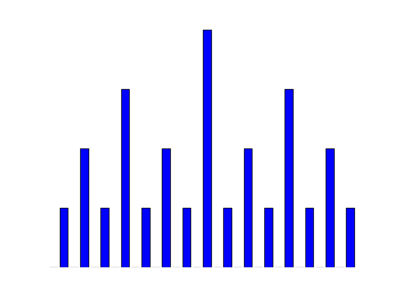
The ruler function graphed.

The mathematical definition for the ruler function is given by $R(n) = k$ where $k$ is the largest number such that $2^k$ divides $n$ . If you like bits and binary strings, you can think of $R(n)$ as the number of zeros on the very right of the binary representation of $n$ , before any ones are encountered.

To see the self-similarity here, let's take a moment and think of the slightly harder version of Hilbert's infinite hotel puzzle, in which an infinite bus shows up with an infinite sequence of guests, each needing a room in the already full infinite hotel. One possible solution to this puzzle relies on the following self-similarity of the natural numbers: if you take every natural number, multiply them by two, and then go through them and insert the correct odd number in between the now all-even numbers, you end up back with the natural numbers. That is, you multiply by two to get all the even numbers, then you insert the odd numbers in between them.

Noting that the zeros in the ruler function are at exactly where the odd numbers are in the natural numbers, and based on the above mentioned self-similarity of the natural numbers, we can come up with a self-similarity for the ruler function: if you increment the numbers in the ruler function by one, and then insert zeros in between each two adjacent numbers, you end up with the ruler function again.

To use this self-similarity to define the ruler function, first we write a function alternate that given two infinite lists, returns an infinite list with elements alternating between the two given lists.

alternate xs ys = head xs : head ys : alternate (tail xs) (tail ys)

Now, all we have to do is use the zeros list that we defined in the first example, and the alternate function above to define the ruler function:

ruler = alternate zeros (map (1 +) ruler)

The same solution translated to Python using coroutines is given below. The alternate generator takes two generators and alternates between them.

def alternate(xs, ys):
    while True:
        yield next(xs)
        yield next(ys)

Then the ruler function is defined similar to the Haskell solution:

def ruler():
    yield from alternate(zeros(), map(lambda x: x + 1, ruler()))

Note that the Python solution assumes Python 3's map behaviour, which returns an iterator. In Python 2, itertools.imap should be used instead.

Kleene Closure

The Kleene closure of a set $S$ is the set of all strings with $S$ as the alphabet. It's usually written as $S^*$ . For example, the Kleene closure of $S = \{0, 1\}$ is given below.

""
"0"
"1"
"00"
"10"
"01"
"11"
"000"
"100"
"010"
"110"
"001"
"101"
"011"
"111"
...

Yet again, let's see if we can find a self-similarity. Here, if we take the Kleene closure of an alphabet, and prepend the empty set or any single character in the alphabet to it, we end up with the Kleene closure again (this is why it's called a closure after all; the set is closed under concatenation!) Let's use this self-similarity to define the Kleene closure now.

kleene a = [] : [x : ys | ys <- kleene a, x <- a]

And the result:

> take 15 $ kleene "01"
["","0","1","00","10","01","11","000","100","010","110","001","101","011","111"]

Note that the Haskell version can be used with both strings and lists (try take 15 $ kleene [0,1]). Also note that while mathematically equivalent, computationally the order in which we do the comprehension is important—switching the order results in the sequence "","0","00","000","0000", ... being generated, never reaching any strings with a one in them.

Let's try to translate this to Python now. Since Python treats strings and lists slightly differently ("" is not the same as [] in Python, but in Haskell "" is the same as [] :: [Char]), we will just write a solution for strings. Writing one for lists would be identical, just replace empty string with empty list.

def kleene(a):
    yield ""
    for s in kleene(a):
        for c in a:
            yield c + s

Exercise: Write a Python solution that does not recursively create generator instances.

Fibonacci Strings

The set of Fibonacci strings is the set of all binary strings which do not contain two consecutive ones (i.e. 11 is a forbidden word). A solution very similar to the Kleene closure solution above exists and is given below. The solution should make the self-similarity obvious.

fibs = "" : [p ++ ys | ys <- fibs, p <- ["0", "10"]]

Let's try it in Python:

def fibs():
    yield ""
    for s in fibs():
        yield "0" + s
        yield "10" + s

Exercise: Write a Python solution that does not recursively create generator instances.

Primes Using The Sieve of Eratosthenes

Now, let's try generating all primes using the sieve of Eratosthenes. This example is different from all the previous ones in that it does not explicitly depend on a self-similarity, but it's a very good example of the power of lazy evaluation or coroutines.

The idea of the sieve is that as soon we find a prime, all multiples of it can be ruled out as primes. To implement this idea in Haskell, first define a filterOutDivisibleBy function that given a number p and a list of numbers filters out any elements in the list that are divisible by p. For example, filterOutDivisibleBy 2 [2,3,4,5,6,7] = [3,5,7].

filterOutDivisibleBy p xs = filter (\x -> x `mod` p /= 0) xs

Now we define a function sieve which given a list, uses filterOutDivisibleBy to filter out everything divisible by the first element in the list (except for the first item itself), then recursively do the same to next remaining list.

sieve (p:xs) = p : sieve (filterOutDivisibleBy p xs)

Then the list of primes is simply sieve called with the appropriate infinite list:

primes = sieve [2..]

Now let's do the same in Python. We will use itertools.count(2) as a translation for Haskell's [2..].

def filter_out_divisible_by(p, xs):
    for x in xs:
        if x % p != 0:
            yield x


def sieve(xs):
    p = next(xs)
    yield p
    yield from sieve(filter_out_divisible_by(p, xs))


def primes():
    yield from sieve(itertools.count(2))

A More Advanced Structure: Free Groups

To finish the article, let's now apply what we've learned so far to a more advanced example. Even if you are not familiar with group theory, this example should be relatively easy to follow. First, the mathematical definition of the set we are generating. Given a set of generator symbols $S$ , first, for each symbol in $S$ the inverse symbol. We will denote the inverse of $a \in S$ by $a^{-1}$ . Denote the extended inverse symbols by $S^{-1}$ . The free group over $S$ , denoted by $F_S$ is then defined as the set of strings with $S \cup S^{-1}$ as the alphabet, with the added constraint that no symbol and its inverse can be adjacent, because they would cancel each other out (most mathematical definitions would use equivalence clasess instead, but to keep it simpler, I just picked a canonical representative from each equivalence class here). The group operation is string concatenation, with cancellation accounted for.

Let's look at an example. Say $S = \{a, b\}$ . Then $S^{-1} = \{a^{-1}, b^{-1}\}$ and

The empty string is written as $\epsilon$ in the list. As an example of the group operation, using the multiplicative notation, we have:

A nice way of visualizing the free group is using a Cayley graph. The Cayley graph for the free group over $S = \{a, b\}$ , which has an interesting fractal structure, is shown below. The basic idea is to think of the two generator symbols $a$ and $b$ as movements to the right, and up, respectively. Their inverses then represent movements to the left and down. However, instead of thinking of the movement as movement along a fixed grid, the distances keep reducing in new directions so as to ensure no two distinct paths (after cancellation is taken into account) ever end up at the same point. Each vertex of the graph is an element of the group then.

The self-similarity in the structure is very evident once visualized as a Cayley graph, and is reminiscent of many organisms found in nature.

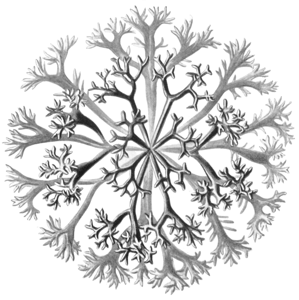
Self-similarity in Chondrus Crispus, commonly known as Irish moss. Drawing by Ernst Haeckel. Source: Wikimedia Commons: Chondrus Crispus.

Let's start to think about how to implement this infinite fractal structure in Haskell. First, for the rest of this section, we will simplify things by hard coding $S = \{a, b\}$ . Generalizing the solution to a given generator set is left as an exercise at the end. Secondly, to simplify the notation, we will use $a^{-1} = A$ and $b^{-1} = B$ . Following this notation, the set we want to generate has the following elements:

"", "a", "b", "A", "B", "aa", "ab", "aB", "AA", "Ab", "AB", "Ba", ...

This listing corresponds to the listing given above in the mathematical notation. In other words, this is the Kleene closure of $S = \{a, b, A, B\}$ minus all strings which have the lower-case and upper-case of the same letter adjacent.

Now, how do we represent the structure? One approach would be to simply use strings, like we did in the Kleene closure example. With that, the self-similarity is also similar to the Kleene closure example: If we take the free group $F_S$ and prepend any generator symbol or its inverse to the beginning, provided we do not put a symbol next to its inverse, we end up back with the set, as if nothing changed. To make the implementation a bit simpler, we will leave out the empty string. This gives us the following implementation:

import Data.Char

isInverseOf x y = x /= y && toUpper y == toUpper x

free_2 = ["a", "b", "A", "B"] ++
         [x:ys | ys <- free_2, x <- ['a','b','A','B'],
                 let y = head ys in not $ isInverseOf x y]

Example use:

> take 15 free_2
["a","b","A","B","aa","ba","Ba","ab","bb","Ab","bA","AA","BA","aB","AB","BB","aaa","baa","Baa","aba"]

Exercise 1: Implement a coroutine-based solution in Python.

Exercise 2: Generalize the solution to free groups generated by an arbitrary set of distinct lowercase letters.

Conclusion and References

As mentioned in the introduction, the point of the article was to explore generating infinite structures using Haskell's lazy evaluation and Python's generators, mostly using the power of self-similarity. Now that you have seen a few examples, maybe you can think of your own examples where this approach is applicable. Finally, as exercise, you can try to implement other infinite structures, such as an infinite tree, using the same idea.

The LiteratePrograms wiki has a nice article on Sieve of Eratosthenes which goes into a lot more detail than I did here. The ruler function example comes from an exercise I was given in a Haskell course. I did some searching but couldn't find a good source for it. If I you happen to know the source, feel free to let me know in the comments.